Case Study: Cleaning a Messy Customer Dataset Before You Analyse It
A deliberately damaged 110-row dataset taken through exploratory data analysis in Inference Stats: duplicate rows, missing values hiding as text, transposed dates, and four imputation methods compared on the same column.
Most analyses fail before the first test is run. Not dramatically — the software returns a number either way. They fail quietly, in the half hour nobody documents: the half hour where duplicates were not checked, missing values were not really missing, and a date column was trusted.
This walkthrough takes a small, deliberately damaged dataset through that half hour. It is a practice file — duplicates, gaps and date faults were introduced on purpose — which makes it useful precisely because we can check whether the cleaning found what was planted. Everything below runs on the free tier: the data tools, Explore, and the graph builder.
The data
110 rows, 8 columns of customer purchase records: Customer_ID, Age, Gender, City,
Salary, Purchase_Amount, Is_Member, Purchase_Date.
Small enough to check by hand, which is the point — every claim below can be verified against the file rather than taken on trust.
Step 1 — the count that decides everything
Before any analysis, one number matters more than the rest: how many rows are actually usable. Run Check my data on the raw file and the scorecard says 110 rows, 8 columns, and 51% complete cases.
Fifty-six rows look complete. Eighteen are.
That gap is the whole lesson of this case study, so it is worth being precise about where it comes from.
Step 2 — the missing values that don't look missing
Three columns — Gender, City and Is_Member — contain no empty cells at all. What
they contain instead is the literal three-letter text nan.
This is not exotic. It is what pandas writes when you export a table with
df.to_csv() and the column holds anything other than pure numbers. The file is
syntactically perfect; the missing values have simply been spelled out as a word.
Left alone, the consequence is specific and silent:
| Column | Empty cells | Cells reading nan |
Truly missing |
|---|---|---|---|
| Gender | 0 | 41 | 41 (37%) |
| Is_Member | 0 | 34 | 34 (31%) |
| City | 0 | 10 | 10 (9%) |
| Salary | 22 | 0 | 22 (20%) |
| Purchase_Amount | 25 | 0 | 25 (23%) |
| Purchase_Date | 14 | 0 | 14 (13%) |
| Age | 8 | 0 | 8 (7%) |
Gender does not have two levels and 37% missing. It has three levels — Male, Female
and nan — and nothing missing at all, as far as any naive tool is concerned. Every
frequency table counts that third group. Every crosstab gives it a row. Compare purchase
behaviour across genders and you will get a third column of results, sitting there
looking like a finding.
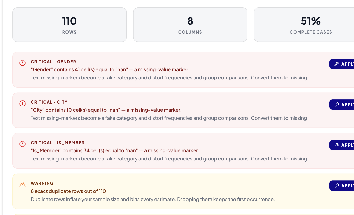
What the health check reports on the raw file. The three critical findings are the disguised missing values; each has a one-click fix. Note the scorecard: 51% complete cases, which is the number that is about to change.
Apply those three fixes and the complete-case count falls from 56 to 18 of 110 — from 51% to 16%. That is the honest figure, and a sharp reminder that 84% of these rows have a gap somewhere.
Step 3 — duplicates, and what one of them reveals
The same health check reports two things about duplication, and they are worth reading as a pair:
8 exact duplicate rows out of 110. Duplicate rows inflate your sample size and bias every estimate. Dropping them keeps the first occurrence.
"Customer_ID" looks like an identifier (91% unique) but has 10 repeated value(s).
Those two numbers do not match, and the mismatch is the interesting part.
Eight rows are byte-for-byte copies. That leaves two customer IDs that appear twice with something different about them. Both are worth looking at directly:
| Customer_ID | Age | Gender | City | Salary | Purchase | Member | Date |
|---|---|---|---|---|---|---|---|
| 1066 | 22 | — | Delhi | 30000 | 1000 | — | 2023-06-02 |
| 1066 | 22 | — | Delhi | 30000 | 1000 | — | 2023-02-06 |
| 1070 | 40 | Male | Bangalore | 70000 | 2000 | Yes | 2023-08-09 |
| 1070 | 40 | Male | Bangalore | 70000 | 2000 | Yes | 2023-09-08 |
Identical in every column but one. And in both pairs, the two dates are the same day with the day and month swapped.
Step 4 — the date fault you cannot see
This is the most dangerous defect in the file, because nothing about it looks wrong.
Every one of the 96 non-missing dates is in ISO YYYY-MM-DD form. There are no mixed
formats to spot, no 13/07/2023 sitting among 07-13-2023. Every value parses. No tool
raises an error. But some of them have had day and month transposed, and
2023-06-02 is every bit as valid a date as 2023-02-06 — it is simply a different one.
The two duplicate IDs are the only reason we know. They are the cases where the same record was entered twice and the transposition happened to only one copy, leaving a matched pair as evidence. Any row where it happened once left no trace at all.
How much of the column could be affected? 42 of the 96 dates (44%) have a day of 12 or lower, which means they read as a valid date under either convention. For those, there is no internal evidence of which reading is right. The remaining 56% have a day above 12 and could only ever be one thing.
No software catches this, including ours. Set the date format in Variable Management and Inference Stats reports 100% parse against ISO — correctly, because every value genuinely is a valid ISO date. There is nothing for a parser to object to.
It is worth being clear about where the tooling does help, because the distinction matters. When a column contains a mixture of readings — some values that can only be D-M-Y sitting beside others that can only be M-D-Y — the app refuses to guess and says so: "Can't tell D-M-Y from M-D-Y — please choose". That catches the common case, where the ambiguity is visible in the formatting. It cannot catch this one, where the transposition happened before the file was written and left the format intact.
This one has to go back to the source. No amount of cleaning recovers information that was destroyed at data entry, and a tool that claimed otherwise would be lying to you.
If the dates matter to your analysis, the honest options are to re-extract the column, or to analyse at a granularity the fault cannot reach — month is no good here, but year is fine, and so is "did this customer purchase at all".
Step 5 — before imputing, ask why the data is missing
The temptation at this point is to reach for an imputation method. One question comes first, because it determines whether imputation is legitimate at all: is the missingness related to anything?
Explore's missing-data diagnostics test each column's missing-indicator against every
other column and report one of three verdicts — Looks random, Related to other
columns, or Not enough data to tell. Nothing here comes back as related. Taking
Salary as the example: it is missing in 14% of Bangalore rows, 21% of Delhi, 23% of
Mumbai and 11% of Pune, and a chi-square across those four gives χ²(3) = 1.55,
p = 0.67. No evidence of a relationship.
Two cautions, both of which apply to every dataset and not just this one:
"Consistent with random" is not "proven random". With 100 rows and four cities, this test would only detect a large imbalance. Absence of evidence is doing a lot of work.
No test can rule out the dangerous case. If high earners decline to state their salary, the missingness depends on the very value that is absent — and there is nothing in the observed data that can reveal it. Inference Stats never claims otherwise; the strongest verdict it offers is Looks random.
Step 6 — four ways to fill a gap, and what each does
Purchase_Amount is the best column to demonstrate on: 25 values missing, and only four
values ever observed — 1000, 2000, 3000 and 4000.
Observed: n = 85, mean 2529.4, median 2000, SD 1171.0.
| Method | Resulting SD | Change | What it actually did |
|---|---|---|---|
| Drop the rows | 1171.0 | — | Kept 85 rows, discarded 25 |
| Impute mean | 1027.9 | −12.2% | Inserted 2529.41, twenty-five times |
| Impute median | 1051.8 | −10.2% | Inserted 2000, twenty-five times |
| Impute mode | 1051.8 | −10.2% | Same as median here (both 2000) |
| kNN (k = 5) | 1051.0 | −10.2% | Borrowed from similar rows |
Two things to take from that table.
Every method narrows the distribution. Filling 25 gaps with a single central value adds 25 observations with no variability, so the spread shrinks by roughly a tenth. Any confidence interval computed afterwards is too narrow, and the p-value that follows is too small. The software will not warn you.
Mean imputation here inserts a value that cannot exist. Purchases in this dataset come in round thousands. The mean is 2529.41. Impute it and the distribution grows a spike of 25 observations at a value that occurs exactly zero times in reality — a fifth of the column, sitting at an impossible number. Inference Stats marks mean imputation with a warning and puts median above it in the list for exactly this reason.
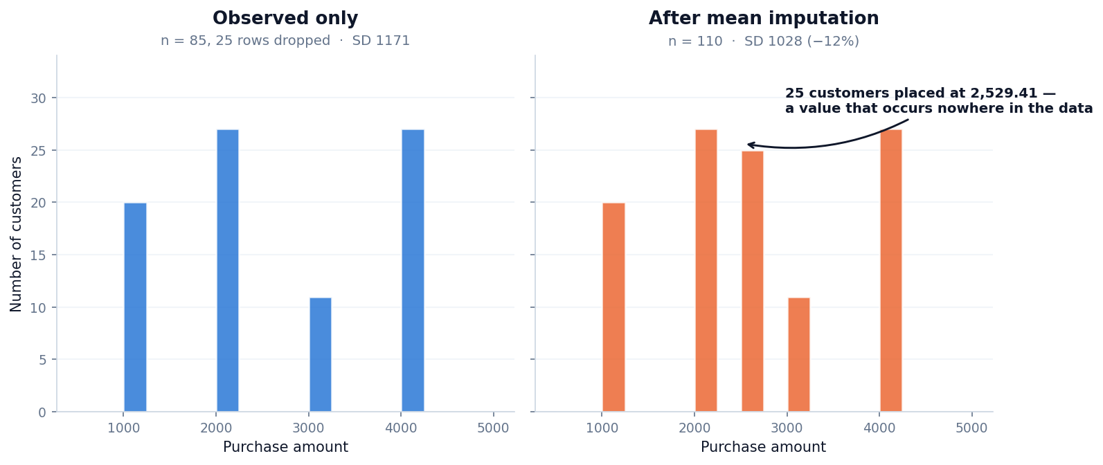
The same column, drawn twice. On the left, the 85 observed values: four amounts, all round thousands. On the right, the same column after the 25 gaps are filled with the mean — a new fifth bar appears between 2000 and 3000, holding more customers than the real 2000 bar does. It is the largest single feature of the imputed distribution and none of it is data. (Both panels are drawn from the dataset itself rather than screenshotted, because the comparison needs the two states side by side.)
Step 7 — why the sophisticated methods do not rescue this
The standard advice is to prefer a method that uses the other columns — regression imputation, or k-nearest-neighbours — over a flat central value. That advice assumes the other columns know something. Here is what they know:
| Age | Salary | Purchase_Amount | |
|---|---|---|---|
| Age | 1.000 | −0.018 | 0.193 |
| Salary | −0.018 | 1.000 | 0.006 |
| Purchase_Amount | 0.193 | 0.006 | 1.000 |
Nothing. Salary and Purchase_Amount correlate at r = 0.006.
Fit the regression the app would fit, predicting Purchase_Amount from Age and
Salary, and it returns R² = 0.05. Its predictions for the missing rows span 2197 to
2971 — a spread that is 21% of the real spread in the observed data. Regression
imputation on this dataset is mean imputation with extra steps and a more convincing name.
kNN does the same: SD −10.2%, indistinguishable from the median.
This is the part worth carrying to your own data. The ranking of imputation methods is not a property of the methods — it is a property of your dataset. Regression and kNN beat the mean when the other columns predict the missing one. Check that they do before choosing, because when they do not, the elaborate method delivers the same shrunken distribution while looking more defensible in the write-up.
What we would actually do with this file
- Drop the 8 exact duplicates. Unambiguous, and they inflate every count.
- Convert
nanto missing in the three text columns. Otherwise a third of the Gender column is a fictional category. - Do not impute the dates. Send them back to the source; analyse by year if that is not possible.
- For a headline estimate, report the complete cases and say how many they are. Eighteen of 110 is a weak dataset, and the right response to a weak dataset is to say so, not to inflate it to 110 with invented values.
- If imputation is needed, use the median, and report that you used it. Not because it is good, but because on this data it is no worse than the alternatives and it is honest about being crude.
What this does not show
This is a practice dataset: the values are drawn from a handful of discrete levels and carry essentially no signal — the strongest correlation in the whole file is 0.19. That makes it ideal for demonstrating cleaning and misleading for anything else. No conclusion about customers should be drawn from it, and none is drawn above.
It also cannot tell you whether your own missing data is random. Nothing can. That question is answered by knowing how the data was collected, not by testing it afterwards.
Running this yourself
Everything here is on the free tier. The data tools check your file and fix what is safely fixable; Explore reports the missing pattern, tests the mechanism and applies the imputation method you choose, showing how many cells each one will change before it changes them; and every step is recorded in a reproducibility log you can export.
Clean your own dataset — free →
Related reading
- Handling missing data — the general treatment of what is skipped over above.
- Which statistical test should I use? — where to go once the data is fit to analyse.
- P-value vs effect size — why the narrowed distribution above matters for what you report.
- Case study: finding phenotypes in VA-ECMO patients — clustering, on data that had already been cleaned.
Written by Dr Hoong Sern Lim MB ChB MD FRCP, Consultant Cardiologist, Queen Elizabeth Hospital Birmingham; Honorary Senior Lecturer, University of Birmingham. ORCID 0000-0002-6569-1805