Case Study: When Customers Leave the Nest — Survival Analysis for Subscription Graduation
A simulated cohort of 446 customers graduated from a managed plan to self-serve, analysed end to end in Inference Stats: Kaplan-Meier, an adjusted Cox model with E-values, an interaction test, restricted mean survival time with a confidence interval, a mixed model of engagement over time, and a cross-validated lasso Cox for variable selection.
Everything in this article is simulated. The two datasets were generated with a seeded script so that they carry a known structure; no real customers, and no real patients, are in them. The design is borrowed from a pattern that clinical registries use constantly — a cohort weaned off a form of support, followed for a composite endpoint, compared across groups, with a repeated measurement over time — because the same toolkit answers the business version of the question. If you run survival analysis on subscribers or on patients, the steps below are the same steps.
Everything below was produced in Inference Stats, with no coding. Every number was checked against the app's own engines before it was written down.
The question
A software company runs a managed "Premium" plan in which an account manager keeps a customer's usage healthy. When usage recovers and stays healthy, the customer is graduated to a self-serve plan: cheaper for the company, and a sign of a customer who no longer needs the support. Some graduated customers thrive. Others close the account, move to an enterprise contract, or ask to go back to Premium — all of which the company counts as failure to stay independent.
Two things are known about each customer at graduation: the channel they were acquired through (paid advertising or organic), and the segment they belong to (consumer or business). The questions are the ones a registry would ask:
- Do business accounts fail to stay independent more often than consumer accounts?
- Does that depend on the acquisition channel?
- Do business accounts also escalate support tickets more, even when they do not leave?
- Does engagement drift after graduation, and differently by segment?
The data
446 customers, one row each, with the segment, the channel, fourteen candidate covariates measured at graduation, the months of follow-up, and the composite event. A second file holds an engagement score (0–100) at months 0, 3, 6, 12 and 24 after graduation, for as long as each customer was still on the plan.
| Customers | 446 — 66 business (14.8%), 380 consumer |
| Acquired through paid channel | 146 (32.7%) |
| Composite events | 183 (41.0%): 77 closed, 76 re-subscribed to Premium, 30 moved to enterprise |
| Follow-up | median 45.8 months (IQR 21.4–77.4), longest 146.8 |
As in the transplant case study, the number that governs the precision of everything that follows is the number of events, not the number of customers. 183 is a reasonable count for a model with five terms; it is not a count that supports fishing.
Step 1 — describe the two groups first
The Comparisons tab runs the Table-1 comparisons — Welch's t-test for continuous covariates (with Mann-Whitney beside it), chi-square for the binary ones. Three differences stand out, and they are the ones you would expect of a business account:
| At graduation | Business (n = 66) | Consumer (n = 380) | p |
|---|---|---|---|
| Licensed seats, mean (SD) | 2.3 (0.6) | 2.0 (0.7) | 0.004 |
| Monthly spend, USD, mean (SD) | 33.3 (12.1) | 24.2 (12.6) | < 0.001 |
| Support tickets last year, mean (SD) | 2.8 (1.7) | 2.1 (1.4) | 0.001 |
| Autopay enabled | 53.0% | 31.1% | < 0.001 |
| Account age, months, mean (SD) | 42.9 (13.4) | 42.6 (13.8) | 0.88 |
| Months on Premium, mean (SD) | 23.2 (12.7) | 20.5 (11.6) | 0.11 |
| Acquired through paid channel | 28.8% | 33.4% | 0.46 |
Business accounts are bigger and busier. They are not older, they did not spend longer on Premium, and they were not acquired differently. That matters for what comes later: any difference in outcome is not obviously explained by when they graduated.
Step 2 — the curves and the log-rank test
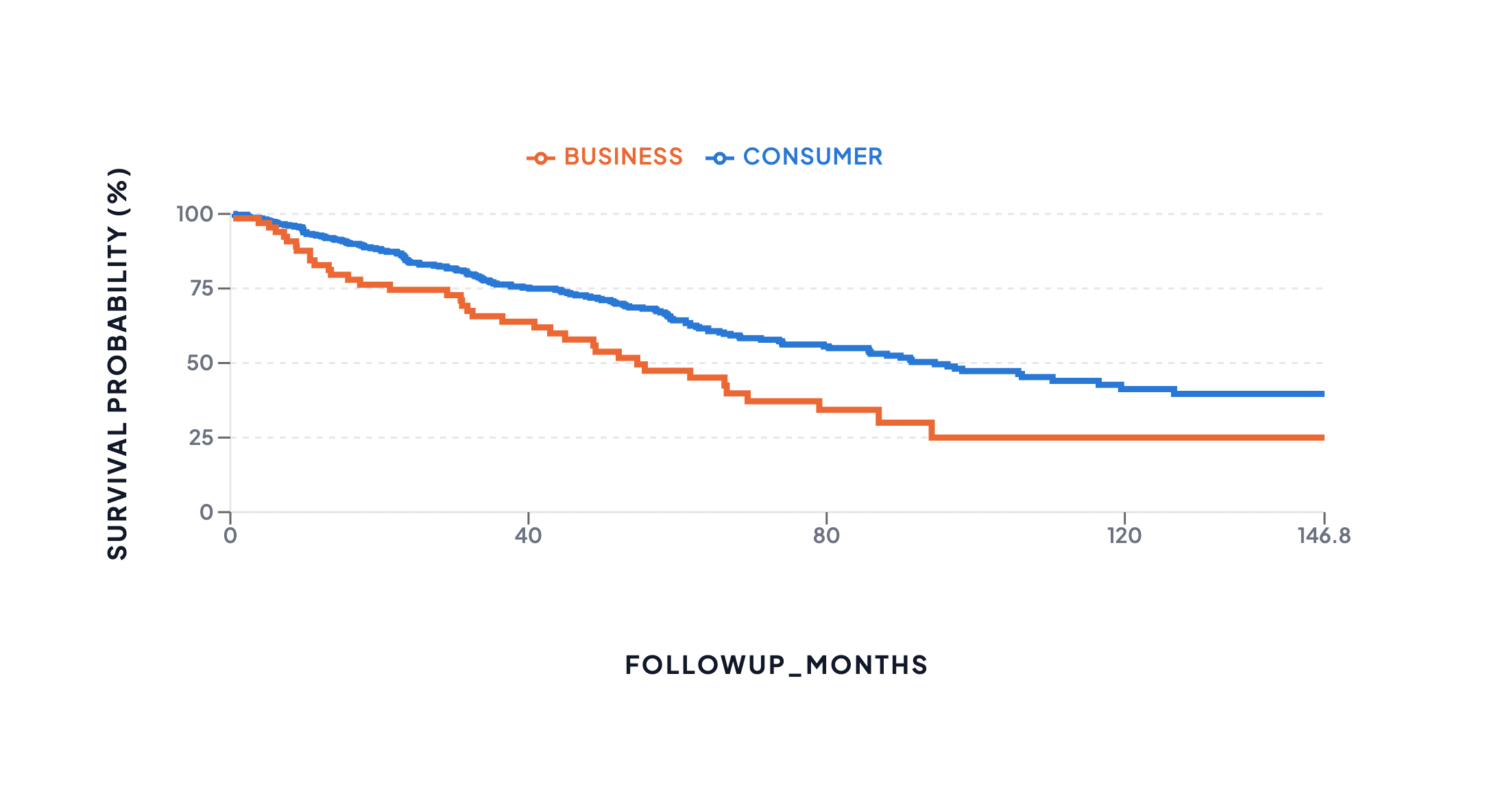
Event-free survival after graduation, by segment, exported from the Survival tab. Orange is business (n = 66), blue is consumer (n = 380). The curves separate within the first year and stay separated.
| Month | Business event-free | Consumer event-free | Business at risk | Consumer at risk |
|---|---|---|---|---|
| 0 | 100% | 100% | 66 | 380 |
| 12 | 82.8% | 92.7% | 51 | 335 |
| 36 | 65.7% | 76.3% | 36 | 219 |
| 60 | 47.4% | 64.3% | 22 | 145 |
| 84 | — | — | 10 | 90 |
| 120 | — | — | 2 | 27 |
The median event-free time is 54.6 months for business accounts and 94.5 for consumer — but read the at-risk table before quoting the second number, because by month 94 the consumer group is down to a few dozen customers and the business group to a handful.
Log-rank χ²(1) = 9.59, p = 0.002
The curves differ, and the difference is not something the log-rank test attributes to chance. That is all it says: it carries no effect size. For that, the Cox model.
Step 3 — the Cox model, unadjusted then adjusted
Setting the group column alone gives the unadjusted hazard ratio. Ticking the prespecified covariates — channel, account age, seats and months on Premium — gives the adjusted one. The three numeric covariates were chosen in advance as the ones most likely to confound a segment comparison; the section "What the original design did that this does not" says why "chosen in advance" is doing real work in that sentence.
A note on how to read the table. Inference Stats dummy-codes a categorical covariate against its first sorted level, and "business" sorts before "consumer", so the app reports the hazard for consumer relative to business:
| Term (adjusted model, n = 446, 183 events) | HR (95% CI) | p |
|---|---|---|
| Segment: consumer vs business | 0.58 (0.40–0.84) | 0.004 |
| Channel: paid vs organic | 0.84 (0.60–1.17) | 0.30 |
| Account age, per month | 1.02 (1.01–1.03) | < 0.001 |
| Seats, per seat | 1.30 (1.05–1.61) | 0.017 |
| Months on Premium, per month | 1.02 (1.00–1.03) | 0.006 |
A hazard ratio of 0.58 for consumer-versus-business is the same fact as 1/0.58 = 1.73 (1.19–2.49) for business-versus-consumer; the interval inverts along with the estimate. The unadjusted version is 1.75 (1.22–2.50). Adjustment barely moves it, which is consistent with the Table 1 finding that the groups were not different on the covariates that plausibly matter.
Channel is not an independent predictor. Paid-acquired accounts have a hazard ratio of 0.84 with an interval that comfortably includes 1. Keep that in mind for step 5.
Step 4 — how strong would an unmeasured confounder need to be?
This is observational data. The company did not randomise anyone to be a business, and the four covariates in the model are the ones that were recorded. Beside every hazard ratio the app now prints an E-value: the minimum strength of association, on the risk-ratio scale, that an unmeasured confounder would need with both the segment and the outcome to explain the estimate away, and the same number for the confidence bound nearer 1.
Because 41% of accounts had the event, the outcome is common, and the app first converts each hazard ratio to an approximate risk ratio before applying the formula — it says so in the panel.
| Term | E-value (estimate) | E-value (CI bound) |
|---|---|---|
| Segment | 2.28 | 1.52 |
| Seats | 1.69 | 1.22 |
| Channel | 1.51 | 1.00 |
The reading: an unmeasured confounder with a risk ratio of at least 2.28 with both segment and outcome would be needed to explain the segment effect away entirely, but one of only 1.52 would suffice to move the interval across 1. The second number is the one a sceptic cares about, and 1.52 is not a large ask — a confounder of that strength is entirely plausible in customer data (the size of the company the account belongs to, say, which this dataset does not record). The E-value does not tell you whether such a confounder exists. It tells you how much of an argument you have if someone proposes one.
The channel row makes the other point: its CI-bound E-value is exactly 1, because the interval already includes 1 — no unmeasured confounding is needed for the data to be consistent with no channel effect.
Step 5 — does the segment effect depend on channel?
The paper-style version of this question is a formal interaction, not two subgroup analyses. Inference Stats can now add a segment × channel term to the Cox model, and when it does it reports the nested-model likelihood-ratio test — the model with the term against the same model without it:
Interaction LRT χ²(1) = 1.08, p = 0.30
The subgroup fits, obtained by filtering to each channel and re-running the adjusted model, look far more dramatic than that:
| Within channel | Business vs consumer HR (95% CI) | p | Business accounts (events) |
|---|---|---|---|
| Organic (n = 300, 133 events) | 1.90 (1.25–2.89) | 0.003 | 47 (29) |
| Paid (n = 146, 50 events) | 1.29 (0.59–2.79) | 0.53 | 19 (8) |
It is tempting to write "the segment effect is confined to organically-acquired accounts". The interaction test is what stops you. One subgroup is significant and the other is not, but the difference between the two estimates — 1.90 against 1.29 — is not itself distinguishable from chance, and the paid subgroup rests on eight events among business accounts. Its interval runs from a halving of risk to nearly a tripling. The honest sentence is that the segment effect is clearly present in the organic channel and undetermined in the paid one, and that the study cannot say whether it differs between them.
The app makes the general form of this mistake hard to commit by accident: the interaction panel says in so many words that when the term is in the model the main-effect hazard ratios describe the reference level only.
Step 6 — check the assumption everything above relies on
Every hazard ratio in steps 3 to 5 assumes proportional hazards. The Schoenfeld residual test runs alongside the model:
Global χ²(5) = 5.18, p = 0.40 — and for segment alone, χ²(1) = 0.02, p = 0.88.
No evidence against proportionality for any term. Had the segment test failed, the single hazard ratio would have been an average over a moving target, and the right thing to report would have been the next step on its own.
Step 7 — restricted mean survival time, now with an interval
RMST answers the question in units a product manager already uses: over the first five years, how many months on average did each group stay independent? The horizon of 60 months was set before looking at the curves, and both groups still have customers at risk there (22 business, 145 consumer).
| At 60 months | RMST, months (SE) | 95% CI |
|---|---|---|
| Consumer | 49.3 (0.96) | 47.4–51.2 |
| Business | 42.5 (2.68) | 37.3–47.8 |
| Difference, business − consumer | −6.8 | −12.3 to −1.2, p = 0.017 |
Until this release the tab reported one restricted mean per group and left the difference to the reader, without an interval; it now computes the difference with a Greenwood-type standard error — the same variance R's survRM2 uses — and a p-value. Over five years, business accounts stayed independent for nearly seven months less on average, and the interval, though wide, excludes zero. This needs no proportional-hazards assumption at all, which is why it is the number to fall back on when step 6 fails.
Step 8 — the secondary endpoint: support escalation
Staying on the plan is not the only thing the company cares about. A second time-to-event outcome — the first escalated support ticket, censored when the customer leaves — is analysed the same way, with segment and channel in the model.
Business vs consumer: HR 2.45 (1.75–3.45), p < 0.001 — E-value 3.11 (2.30 for the bound). Channel: HR 1.15 (0.87–1.53), p = 0.32.
Business accounts escalate at about two and a half times the rate, and this effect is robust to a considerably stronger unmeasured confounder than the primary one was. Put next to the event-type breakdown — 24% of business accounts closed outright against 16% of consumer accounts, and 26% re-subscribed to Premium against 16% — the picture is of a segment that needs more support than the self-serve plan provides, rather than one that simply leaves.
Step 9 — engagement over time: the mixed model
The second file has 2,012 engagement scores from the 446 customers, up to five per customer. Scores from the same customer are not independent, so the Regression tab's mixed model fits a random intercept per customer, and — new in this release — accepts a month × segment interaction, so that each segment gets its own slope, and draws the fitted trajectories.
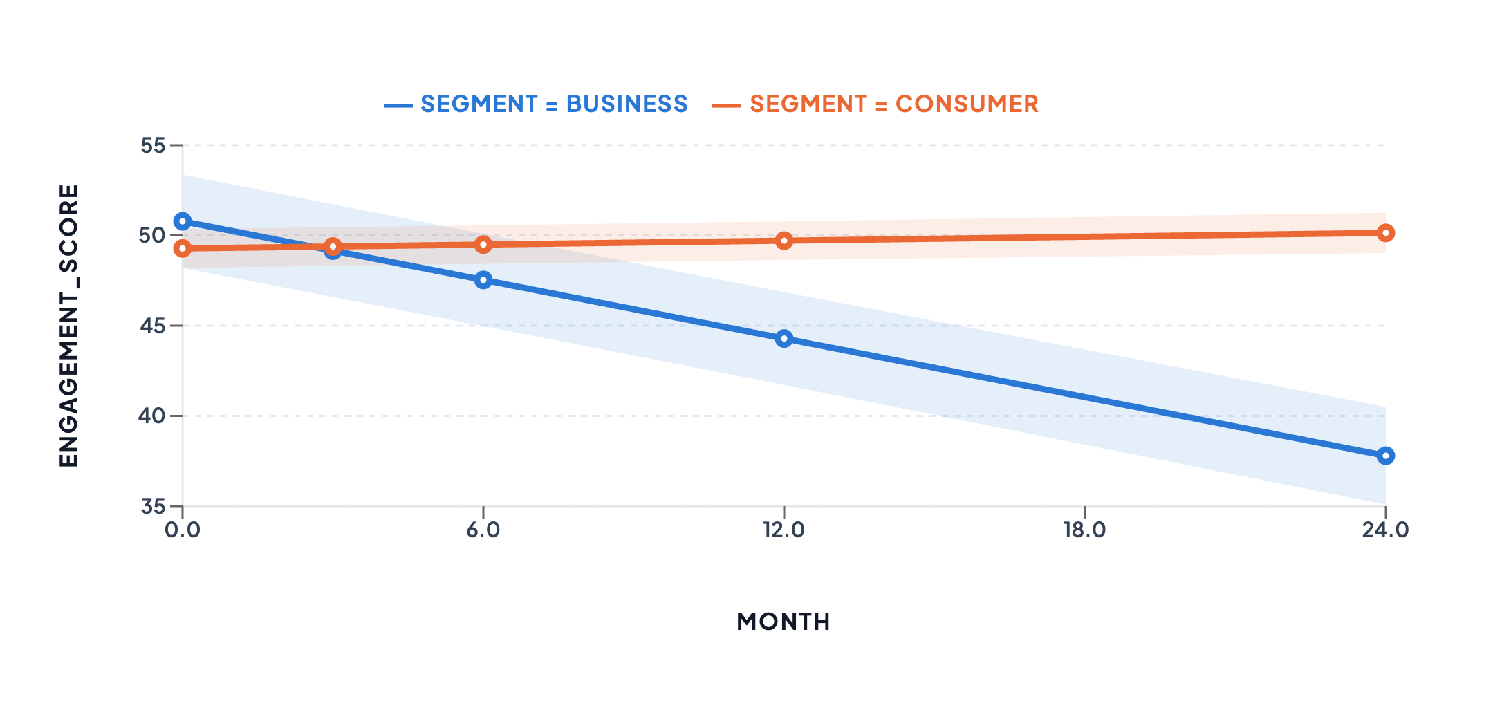
Fitted engagement score by month since graduation for each segment, with 95% bands from the full coefficient covariance, exported from the Regression tab. Blue is business, declining; orange is consumer, flat.
| Fixed effect | Estimate (95% CI) | p |
|---|---|---|
| Intercept (business, month 0) | 50.8 (48.2 to 53.4) | < 0.001 |
| Month (business slope) | −0.54 (−0.59 to −0.49) per month | < 0.001 |
| Segment: consumer (difference at month 0) | −1.5 (−4.3 to 1.3) | 0.29 |
| Month × consumer (difference in slope) | +0.58 (0.52 to 0.63) per month | < 0.001 |
ICC 0.90: nine-tenths of the variation in engagement is between customers, which is exactly why a model that ignored the clustering would have got its standard errors wrong.
The interaction row is the finding. With the interaction in the model, the "month" row is the business slope (the reference level): engagement falls by about half a point a month, some thirteen points over two years. The consumer slope is −0.54 + 0.58 ≈ +0.04 a month — flat. The segment row is the difference at month zero, and it is small and undetermined: the two groups graduate at the same level of engagement and then diverge. Fit the same model without the interaction and the story disappears — a single pooled slope of −0.04 a month and a segment difference with p = 0.06 — because the average of a flat line and a falling one is a slightly falling one.
Two cautions. The scores after leaving are absent by construction, so the later months (313 customers at month 24 against 446 at month 0) are the customers who stayed; the trajectory is for customers still on the plan, not for the cohort. And these are within-customer (conditional) slopes, which for a linear mixed model happen to coincide with the population-average ones — the app says so on the plot, because for a logistic mixed model they would not.
Step 10 — letting the lasso choose
The clinical pattern this case study mirrors did not prespecify its adjustment covariates. It handed all of its candidates to a LASSO-penalised Cox model under cross-validation, kept whatever survived, and then ran the prespecified model as a sensitivity analysis. Inference Stats now fits that model too — the "Variable selection (lasso Cox)" switch under the covariates, verified against R's glmnet — so the case study can do it in the paper's order rather than only in the app's.
Sixteen candidates went in: the fourteen covariates measured at graduation, the channel, and the segment. Each was standardised, so the penalty treats a spend in dollars and a score out of ten alike, and the penalty strength λ was chosen by ten-fold cross-validation. The app reports two λs, and on this cohort they tell very different stories:
| Rule | λ | Kept |
|---|---|---|
| 1-SE (the default) | 0.113 | none — the null model |
| Minimum CV deviance | 0.033 | six: account age, seats, months on Premium, storage, autopay, segment |
The 1-SE rule keeps the simplest model whose cross-validated deviance is within one standard error of the best. Here the curve is nearly flat: the best λ improves on the null model by 0.065 units of deviance against a standard error of 0.44, so the rule cannot distinguish "these six covariates" from "no covariates at all" and returns the latter. That is not a failure of the method. It is the method reporting, correctly, that 183 events do not determine which of sixteen candidates predict the hazard — a "kept set" from λ-min should be read in that light.
At λ-min the six survivors include the three the prespecified model was built on (account age, seats, months on Premium), which is reassuring, plus storage, autopay and the segment itself — with shrunken hazard ratios of 1.24, 1.09 and 1.13 per standard deviation for the first three, and 0.90 for consumer-versus-business. Those are smaller than the ordinary model's, deliberately: shrinkage is the price of selection, and the app labels them as such. It also prints no p-values, intervals or Schoenfeld test for this fit, for the same reason its penalised logistic regression prints none: the model chose its own covariates from this outcome, and the usual standard errors assume it did not. A button refits the ordinary Cox model on the kept set for convenience, with a warning that its p-values are post-selection.
Two lessons carry over to the paper's setting. Selection is for prediction and parsimony, not a verdict on what matters causally — a candidate correlated with a kept one is dropped whether or not it matters. And the kept set is unstable at small event counts; the paper's smaller subgroup had fewer than sixty patients, which is exactly where a lasso's choices change with a handful of rows. Reporting the prespecified model beside the selected one, as the paper did and as steps 3 to 9 do here, is the honest design.
The story, in one paragraph
No channel difference in staying independent. Business accounts regress to a managed plan about 1.7 times as fast (1.19–2.49), stay independent nearly seven months less over five years (1.2–12.3), and escalate support tickets at 2.5 times the rate — and their engagement declines by half a point a month after graduation while consumer accounts hold steady. Whether the segment effect is confined to the organic channel is the question this cohort cannot answer: the subgroup estimates differ, the interaction test does not (p = 0.30), and the paid subgroup rests on eight events. An unmeasured confounder of modest strength (risk ratio 1.5) could move the primary interval across 1, and handed all sixteen candidates, a cross-validated lasso keeps either nothing or six of them depending on the rule — the events do not settle which covariates predict the hazard, and a prespecified model is the sturdier claim.
Running this yourself
Both files are in the repository under marketing/figures/datasets/, together with the
seeded script that generated them. The Survival tab takes the cohort file: time
followup_months, event composite_event, group segment, Cox covariates channel,
account_age_months, seats and months_on_premium, an interaction of segment and
channel, and an RMST horizon of 60. For step 10 tick all fourteen covariates and
channel, then switch on "Variable selection (lasso Cox)" and compare the two λ rules. Filter rows by channel in the Data tab for the
subgroup fits. The Regression tab takes the monthly file: Mixed Model, outcome
engagement_score, predictors month and segment, cluster customer_id, and the
month × segment interaction.
Run it on your own data → — Survival analysis and the mixed model are part of Pro. A free account gets you the data tools, Explore and group comparisons, so you can load your file and build Table 1 before deciding.
Or read up on the methods first: Kaplan-Meier estimator · log-rank test · Cox proportional hazards · E-value · lasso Cox regression · restricted mean survival time
Related reading
- Case study: survival after heart transplant — the clinical sibling: the same toolkit on a real cohort, where the answer was "undetermined".
- P-value vs effect size — why "significant in one subgroup, not the other" is not an interaction.
- Competing risks in survival analysis — what to do when the three event types should not be pooled.
- Which statistical test should I use? — the decision guide this sits under.
Written by Dr Hoong Sern Lim MB ChB MD FRCP, Consultant Cardiologist, Queen Elizabeth Hospital Birmingham; Honorary Senior Lecturer, University of Birmingham. ORCID 0000-0002-6569-1805