Interpreting Competing Risks in Survival Analysis (Why 1−KM Overestimates)

Competing risks explained: why 1−Kaplan-Meier overestimates event probability, when to use cumulative incidence functions, and how to interpret them — with examples.

If your patients can experience more than one kind of event — death before transplant or transplant, relapse or death in remission, hospital discharge or in-hospital death — you have competing risks. And if you analyze that data with a standard Kaplan-Meier curve, you will systematically overestimate every risk you report. Here's why, and what to do instead.

What is a competing risk?

A competing risk is an event that prevents your event of interest from ever happening. A patient on the transplant waiting list can die before transplant (the event you're studying) or receive a transplant (after which "death before transplant" is no longer possible). Transplant isn't just missing data about that patient — it's an event that removes them from risk entirely.

That distinction matters because Kaplan-Meier has exactly one way to handle patients who leave: censoring. And censoring carries a hidden assumption — that censored patients go on to experience the event at the same rate as those still being followed. A transplanted patient does not go on to die-before-transplant at any rate. The assumption is not just violated; it's impossible.

What goes wrong: 1−KM inflates the risk

When you treat the competing event as censoring and report 1−KM as "probability of death before transplant," the curve redistributes the transplanted patients' future risk onto everyone else — counting risk for patients who can no longer have the event. The result:

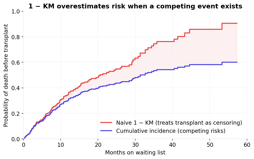
In this simulated waiting-list cohort, the naive 1−KM curve (red) reports a 5-year "risk" approaching 90%, while the correct cumulative incidence function (blue) tops out near 60%. The shaded gap is pure artifact. Published analyses have overstated risks by 20–30% this way, and the error always points the same direction: too high.

The fix: cumulative incidence functions

The cumulative incidence function (CIF, estimated by the Aalen-Johansen method) answers the question you actually asked: what is the probability that this event happens by time t, in a world where the competing event also happens? Each event type gets its own curve, and — unlike stacked 1−KM curves, which can sum to more than 100% — CIFs for all events sum correctly:

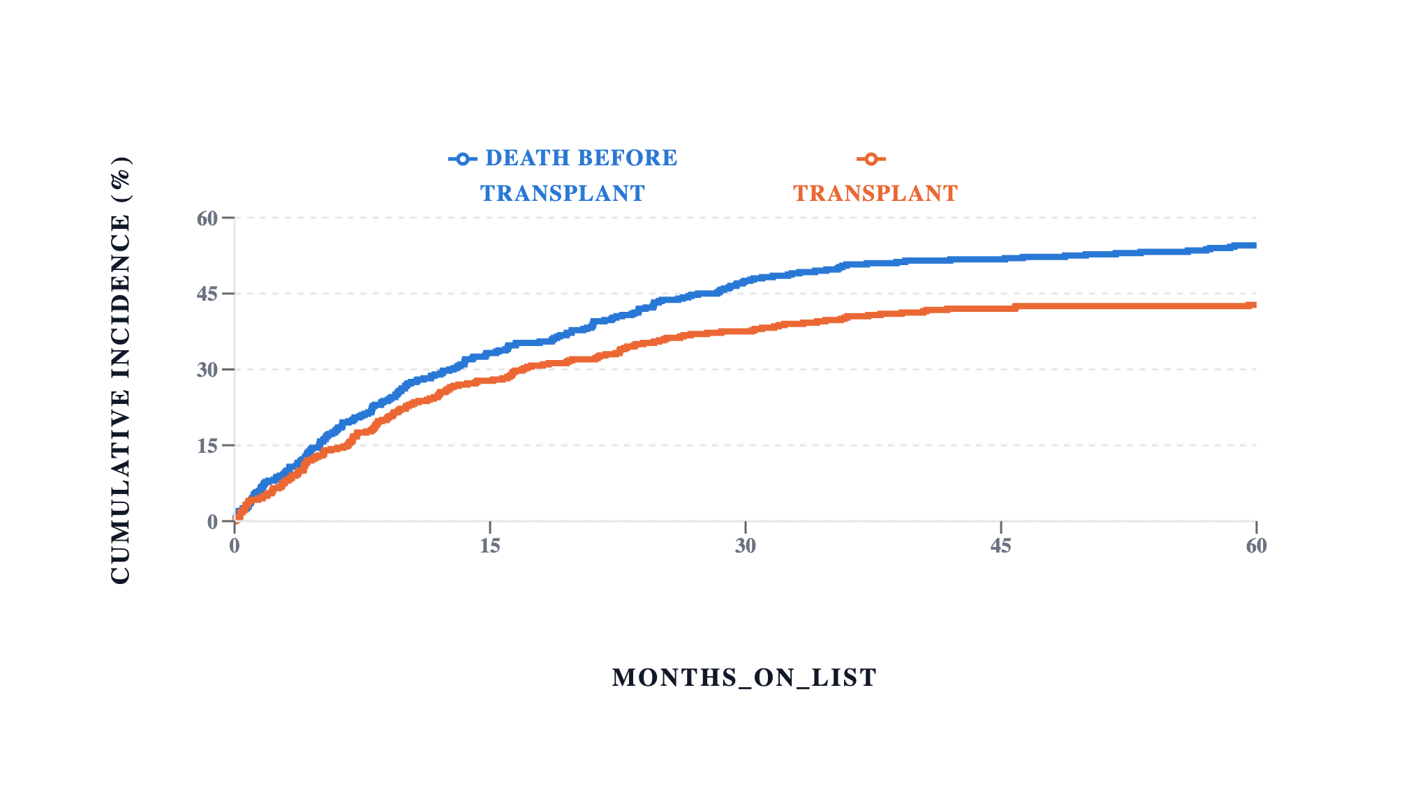
Read the blue curve directly: by 24 months, 42% of listed patients had died before transplant. Read the orange curve the same way: 35% had been transplanted. Add them and you get 77% — the probability that something has happened by two years, leaving 23% still on the list. Do it again at the right-hand edge and the curves give 55% and 43%, summing to 97%: close to certainty, and still under it. That sum staying below 100% is the internal consistency check 1−KM fails.

Note the shape, too. Both curves are steep early and flatten as follow-up lengthens, because each one is competing for the same shrinking pool of patients still waiting. A CIF that climbs in a straight line to the end of follow-up is usually a plotting artefact rather than a finding.

How to interpret (and report) competing-risks results

Three rules keep you honest. First, report CIFs, not 1−KM, whenever a competing event exists — and say so in Methods ("cumulative incidence was estimated accounting for X as a competing risk"). Second, know which question you're answering: CIFs (and Fine-Gray models) describe real-world probability — right for prognosis and planning; cause-specific hazard models describe etiology — right for "does this biomarker drive relapse?" The two can genuinely disagree, because a treatment that increases transplant rates mechanically lowers the incidence of death-before-transplant without touching the death hazard. Third, when comparing groups, remember a difference in one event's CIF can be driven by the other event's rate — always show both curves.

When is plain KM fine? When the competing event is negligible (<5% of subjects) or when your endpoint is all-cause ("death or transplant, whichever first"). All-cause mortality has no competing risk, which is one reason it remains the cleanest endpoint in trials.

Run a competing-risks analysis in two minutes

Inference's Survival module includes Kaplan-Meier, log-rank, Cox, RMST, and cumulative incidence for competing risks — you define your event codes (e.g. 1 = death, 2 = transplant, 0 = censored), and it plots the CIF per event with point estimates at any time you choose. Every method is validated against the reference implementation in Python's lifelines. The Guided flow will route you here automatically if you describe a time-to-event question, and warn you when your event column has more than two codes.

Upload your survival data and get the right curve → — the Survival module is part of Pro; a free account covers the data tools, Explore and group comparisons.

Related reading

• Which statistical test should I use? — the decision guide this article sits under.
• Handling missing data — censoring versus missingness, and why they need different treatment.
• P-value vs effect size — a hazard ratio is an effect size; report it with its interval.
• Kruskal-Wallis vs ANOVA — comparing a non-time-to-event outcome between the same arms.

References

The methods on this page are not our inventions — these are the primary sources. Where a claim here is contested in the literature, the reference is the place to check it rather than take our word for it.

• Fine, J. P., & Gray, R. J. (1999). A proportional hazards model for the subdistribution of a competing risk. Journal of the American Statistical Association, 94.
• Putter, H., Fiocco, M., & Geskus, R. B. (2007). Tutorial in biostatistics: competing risks and multi-state models. Statistics in Medicine, 26.
• Austin, P. C., Lee, D. S., & Fine, J. P. (2016). Introduction to the analysis of survival data in the presence of competing risks. Circulation, 133.
• Andersen, P. K., Geskus, R. B., de Witte, T., & Putter, H. (2012). Competing risks in epidemiology: possibilities and pitfalls. International Journal of Epidemiology, 41.

FAQ

Is censoring always wrong? No — administrative censoring (end of study, loss to follow-up) is exactly what KM is for. Censoring is wrong only for events that make your endpoint impossible.

CIF or Fine-Gray or cause-specific Cox? CIF describes; the other two model covariates. Use Fine-Gray for prediction/prognosis questions and cause-specific Cox for etiological questions — and consider reporting both.

Can the CIF ever exceed the 1−KM estimate? No. 1−KM is always ≥ the CIF; equality holds only when there are no competing events.

Do I need special software? You need Aalen-Johansen estimation — standard KM tools won't do it. Inference, R (cmprsk/survival), and Stata (stcompet) all can; base SPSS cannot without extensions.

Written by Dr Hoong Sern Lim MB ChB MD FRCP, Consultant Cardiologist, Queen Elizabeth Hospital Birmingham; Honorary Senior Lecturer, University of Birmingham. ORCID 0000-0002-6569-1805

All guides · About the author · How we validate