Case Study: Survival After Heart Transplant, With and Without a Mechanical Bridge

A real heart-transplant cohort analysed end to end in Inference Stats: Kaplan-Meier curves, a log-rank test, a Cox hazard ratio and restricted mean survival time at one year — and what to conclude when the p-value is 0.69.

Most survival analyses people publish found something. This one did not, which makes it the more useful worked example — because the hard part of survival analysis is not producing a curve, it is knowing what you are allowed to say when the curves sit on top of each other.

Everything below was produced in Inference Stats from a clinical dataset, with no coding.

The question

Some patients waiting for a heart transplant deteriorate before an organ becomes available and are supported on short-term mechanical circulatory support — a pump that takes over some of the circulation — to keep them alive until one does. They reach the operating theatre in a different state from patients who waited without one.

The question is whether being bridged that way is associated with worse survival after the transplant.

The data

273 heart transplant recipients, each with three fields: days of follow-up, whether the patient died, and whether short-term mechanical support was used as a bridge.

No bridge: 197 patients, 29 deaths
ST-MCS bridge: 76 patients, 10 deaths

Follow-up runs to just over six years, with a median of 887 days. 39 deaths in total.

That last number is the one that governs everything that follows. In survival analysis the precision of your answer is set by the number of events, not the number of patients — 273 people sounds substantial, but 39 deaths is a small study.

Step 1 — the curves

Kaplan-Meier is the right starting point because it handles the thing that makes this data awkward: most of these patients are still alive. Someone recruited eight months before the data was extracted has contributed eight months of survival and no death, and throwing them away or counting them as a survivor would both be wrong. Kaplan-Meier counts them for exactly as long as they were observed and then removes them from the denominator.

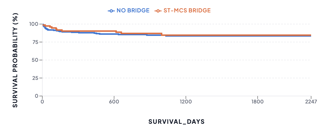
Kaplan-Meier survival curves for transplant recipients with and without a short-term mechanical support bridge

Survival after transplant, by bridging status. Blue is no bridge (n = 197), orange is ST-MCS bridge (n = 76). Both curves drop early and then flatten — the risk is concentrated in the first few months, after which very few patients die. The two lines are within a couple of percentage points of each other throughout.

Two things are worth reading off this figure before any test is run.

The curves are essentially superimposed. Whatever the p-value turns out to be, no test is going to rescue a difference that is not visible.

Neither curve reaches 50%. Survival plateaus in the mid-eighties, so there is no median survival to report in either group — the statistic most people reach for first does not exist here. Keep that in mind; it comes back in step 4.

Step 2 — the log-rank test

The log-rank test asks whether the two curves differ over the whole follow-up period, by comparing the deaths actually observed in each group at each time point against the number expected if bridging made no difference.

χ² = 0.16, p = 0.693

No evidence of a difference.

What that p-value does and does not mean

This is where most write-ups go wrong, in one of two directions. Either the null result gets buried, or it gets reported as though bridging has been shown to be safe.

Running the Cox model makes the problem visible:

HR = 0.87 (95% CI 0.42 to 1.78), p = 0.694

The app's own interpretation panel puts it plainly, unprompted:

"ST-MCS bridge vs No bridge is not statistically significant (p = 0.694) and its hazard-ratio CI [0.42, 1.78] spans 1 — the effect is undetermined, not null."

Read the interval rather than the p-value. It is consistent with bridged patients having less than half the risk of death and it is consistent with them having nearly twice the risk. Both of those would be clinically important, and this study cannot tell them apart. "No significant difference" describes what the test did; "no difference" would be a claim the data does not support.

With 39 events, an interval that wide is the expected result, not a surprise. The honest summary is that the study is too small to settle the question — which is worth saying explicitly, because it points at what a useful next study would need.

Step 3 — read the numbers at risk

Every Kaplan-Meier figure should be read alongside the number of patients still being followed:

Day	No bridge	ST-MCS bridge
0	197	76
449	140	60
899	96	40
1348	59	20
1798	20	3
2247	1	0

The flat right-hand section of the curve rests on almost nobody. By day 1798 the bridged group is down to three patients, so the last stretch of that line is not evidence of anything. This is the single most common way survival figures mislead, and the fix is just to print the table.

Step 4 — restricted mean survival time

Because neither group reaches a median, the usual "median survival was X versus Y" sentence is unavailable. RMST is the alternative, and it is easier to explain than the hazard ratio: pick a time horizon, and RMST is the average time alive up to that horizon — literally the area under the survival curve.

At a one-year horizon:

No bridge: 329.6 days of the possible 365
ST-MCS bridge: 337.6 days
Difference: +7.9 days in favour of the bridged group

That is a statement anyone can act on: over the first year after transplant, the average difference between the two groups is about eight days, in a year. Compare that with trying to explain "hazard ratio 0.87" to a patient. Both come from the same data; only one of them answers the question in units a person recognises.

Two cautions. The horizon is a choice you make, and a different horizon can give a different-looking answer, so state it and state why. And the eight days here carries the same uncertainty as everything else in this analysis — with 39 events, it should not be read as a precise estimate.

Step 5 — check the assumption you relied on

The hazard ratio above assumes proportional hazards: that whatever difference in risk exists between the groups is roughly constant over time, rather than large early and gone later. If that fails, a single HR is an average of things that should not be averaged.

Inference Stats runs the Schoenfeld residual test alongside the model:

χ²(1) = 0.896, p = 0.344 — the assumption looks reasonable.

Worth doing even here. A null result obtained under a violated assumption is not a null result, it is an uninterpretable one — and had the test failed, RMST would have been the right thing to report instead, precisely because it makes no proportional-hazards assumption at all.

What this does not show

This is observational data. Patients are not bridged at random — they are bridged because they deteriorated, which means the bridged group was sicker at the moment the decision was made. Any comparison between the groups is confounded by whatever drove that decision.

That cuts in an interesting direction here. A sicker group with the same survival is not the same finding as two similar groups with the same survival, and this analysis cannot distinguish them. It would need the variables that describe how ill each patient was — and a Cox model that adjusts for them.

The app's Result Companion flags the general form of this itself:

"Cox regression estimates association; causal claims need a designed study."

Running this yourself

The Survival module takes a spreadsheet with a time column, an event column and optionally a group, and returns the Kaplan-Meier curves, the numbers at risk, the log-rank test, a Cox model with its hazard ratios and confidence intervals, the Schoenfeld test for proportional hazards, and RMST at a horizon you set. It also drafts the methods and results sentences for you to check and edit.

Run it on your own data → — Survival analysis is part of Pro. A free account gets you the data tools, Explore and group comparisons, so you can load your file and look at it before deciding.

Or read up on the methods first: Kaplan-Meier estimator · log-rank test · Cox proportional hazards · restricted mean survival time